Simple Linear Regression
1. Import Libraries
# import libraries
import pandas as pd
import numpy as np
import matplotlib.pyplot as plt

from statsmodels.formula.api import ols
import statsmodels.api as sm
2. Load and Verify Dataset
# load dataset and create dataframe
df = pd.read_csv('data/edincome.csv').round(1)
# verify first few records
df.head()
| Education | Income | |
|---|---|---|
| 0 | 10.0 | 32.1 |
| 1 | 10.4 | 36.5 |
| 2 | 10.7 | 23.9 |
| 3 | 11.1 | 52.3 |
| 4 | 11.4 | 30.2 |
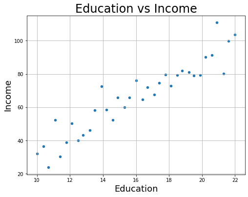
# plot scatterplot

fig = df.plot.scatter(x="Education", y="Income",figsize=(8, 6) )
plt.title('Education vs Income',fontsize=24)
plt.xlabel('Education', fontsize=18)
plt.ylabel('Income',fontsize=18)
plt.grid()
3. Run Simple Linear Regression
slr = ols('Income ~ Education',df).fit()
print(slr.params)
Intercept   -23.176365
Education     5.574237
dtype: float64
slr.params[0]
-23.176364855801438
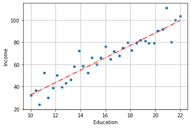
fig = df.plot.scatter(x="Education", y="Income")
x = np.linspace(10,22,100)
y = slr.params[1]*x + slr.params[0]
plt.plot(x, y, '-.r')
plt.grid()
4. Review Results and Evaluate Model
slr.summary()
| Dep. Variable: | Income | R-squared: | 0.878 |
|---|---|---|---|
| Model: | OLS | Adj. R-squared: | 0.875 |
| Method: | Least Squares | F-statistic: | 238.4 |
| Date: | Tue, 25 Jan 2022 | Prob (F-statistic): | 1.17e-16 |
| Time: | 22:45:36 | Log-Likelihood: | -119.61 |
| No. Observations: | 35 | AIC: | 243.2 |
| Df Residuals: | 33 | BIC: | 246.3 |
| Df Model: | 1 | ||
| Covariance Type: | nonrobust |
| coef | std err | t | P>|t| | [0.025 | 0.975] | |
|---|---|---|---|---|---|---|
| Intercept | -23.1764 | 5.918 | -3.917 | 0.000 | -35.216 | -11.137 |
| Education | 5.5742 | 0.361 | 15.440 | 0.000 | 4.840 | 6.309 |
| Omnibus: | 2.854 | Durbin-Watson: | 2.535 |
|---|---|---|---|
| Prob(Omnibus): | 0.240 | Jarque-Bera (JB): | 1.726 |
| Skew: | 0.502 | Prob(JB): | 0.422 |
| Kurtosis: | 3.420 | Cond. No. | 75.8 |
Notes:
[1] Standard Errors assume that the covariance matrix of the errors is correctly specified.
print(slr.rsquared)
0.8784032808796992
print(slr.mse_model)
13766.191657863852
5. Generate Predictions
# predict new points
data = {'Education': [12,16,18]}
df_predict = pd.DataFrame(data).round(1)
df_predict['Income'] = slr.predict(df_predict).round(1)
df_predict
| Education | Income | |
|---|---|---|
| 0 | 12 | 43.7 |
| 1 | 16 | 66.0 |
| 2 | 18 | 77.2 |